I am pulling quarterly financial data and I am wondering if there is a function that will allow me to pull data in while skipping the annual data that occurs every fifth cell. I have seen some suggestions to use offset, but I cannot see how that does anything other than pull in the data from every fifth cell that I am hoping to exclude. Thanks in advance!
23 Answers
Assuming your periods (quarters, years) are in column A and the quarterly values are indicated by Q1, Q2 etc, and that column B contains the amounts. You can try in column C the formula:
=IF(LEFT(A2,1)="Q",B2,"") Drag it to fill the other cells.
It checks if the cell in column A starts with Q. If yes, it copies the content of the corresponding row in column B.

If the raw data doesn't have usable text labels that distinguish a data row from a total row, then add a 'flag' column: =MOD(ROW(B2),5)<>0 will provide a TRUE/FALSE flag that autofilter and pivottable can filter on.
Since OP has not provided the Source data, therefore I've assumed data set, and used method which calculates year wise quarterly total and skips every 5th cell, which is Year Total.
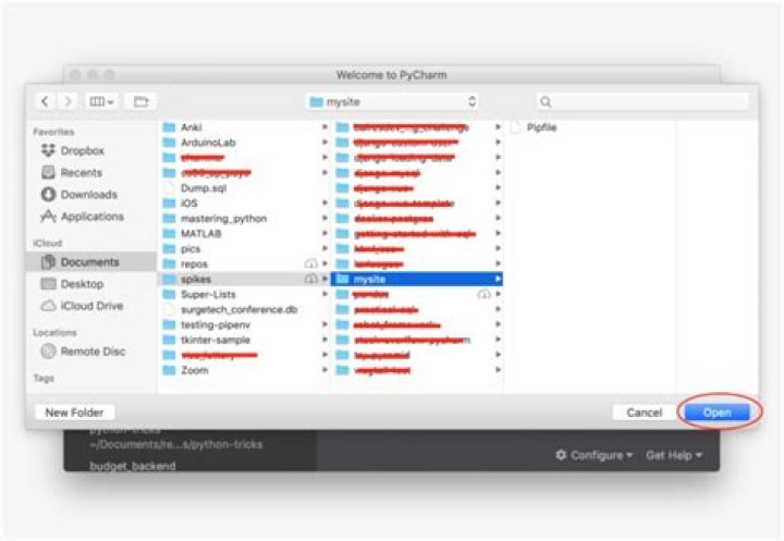
How it works:
Put Quarter Value in Column F as shown.
Formula in cell
G16:=IFERROR(SUMPRODUCT((ROUNDUP(MONTH($A$16:$A$47)/3,0)=MID(F16,2,1)*1)*(YEAR(A$16:A$47)=RIGHT(F16,4)*1)*($B$16:$B$47)),"")
Edited:
In case if you want to generated period of each quarter in column F with Year Total then you need to use these formulas.
Formula in cell D16:
="Q"&INT((MONTH(A16)-1)/3)+1&" "&YEAR(A16)Now this formula in cell F16:
=IF(MOD(ROW(),5)=0,"Year Total:",IFERROR(INDEX($D$16:$D$47,MATCH(0,COUNTIF($I$15:I15,$D$16:$D$47),0)),""))
N.B.
- Since source table doesn't have data for Q3 & Q4 in year 2020, so that the formula returns ZERO in cells G23 & G24.
- You may adjust quarter values in column F, as well as cell references in the formula as needed.